Special example

If \(a_i = 1\) for \(i = 0, 1, 2, \dots\) and \(b_i = 1\) for \(i = 1, 2, \dots\), the recursive formula becomes

\[x_k = x_{k-1} + x_{k-2}\]

and \(n_k\) is the \((k+2)\)-nd Fibonacci number, while \(d_k\) is the \((k+1)\)-st Fibonacci number. The convergents of the continuing fraction

\[1 + \frac{1}{1 + \frac{1}{1 + \frac{1}{1 + \ddots}}}\]

are the ratios of consecutive Fibonacci numbers, and converge to the golden ratio

\[\psi = \frac{1 + \sqrt{5}}{2}\]

Julia implementation

Our continuous fraction coefficients will be functions of a complex variable. We will also want to calculate the convergents for a whole array of complex numbers at once. Both of thee things are easy in Julia.

We want to find convergents of a continuous fraction

\[a_0(z) + \frac{b_1(z)}{a_1(z) + \frac{b_2(z)}{a_2(z) + \frac{b_3(z)}{a_3(z) + \ddots}}}\]

We can consider \(a\) and \(b\) functions of two variables: the index \(i\) and a complex number \(z\):

\[\begin{aligned} a :\ & \mathbb{N}\times\mathbb{C} \mapsto \mathbb{C}\\ b :\ & \mathbb{N}^+\times\mathbb{C} \mapsto \mathbb{C} \end{aligned}\]

We will first define a function drec that will implement the doubly recursive formula. It will receive the coefficient functions \(a\) and \(b\), with signatures Int64 -> T -> T where in our case T will be some sort of complex number or complex number array, two values of type T, representing the “initial values” \(x_{s-2}\) and \(x_{s-1}\), starting index \(s\) that will be the index of the first calculated value, and ending index \(e\) that will be the index of the last calculated value, one that will be returned. Finally, drec will receive as its last argument a value of type T.

The function will use broadcasting versions of operators so it will allow T to be an array.

function drec(a::Function, b::Function, 
              xₛ₋₂::T, xₛ₋₁::T, s::Int64, 
              e::Int64, z::T) where {T}
    for i = s:e
        (xₛ₋₂, xₛ₋₁) = (xₛ₋₁, a(i, z) .* xₛ₋₁ .+ b(i, z) .* xₛ₋₂)
    end
    return xₛ₋₁
end

## drec (generic function with 1 method)

Now we will use the doubly recursive formula to find both the numerator and the denominator of the \(k\)-th convergent. Again, all operators broadcast.

function contfrac(a::Function, b::Function, k::Int64, z)
    n0 = a(0, z)
    n1 = a(1, z) .* n0 .+ b(1, z)
    d1 = a(1, z)
    d2 = a(2, z) .* d1 .+ b(2, z)

    return drec(a, b, n0, n1, 2, k, z) ./ drec(a, b, d1, d2, 3, k, z)
end

## contfrac (generic function with 1 method)

Generating images

We will start by creating a \(500\times 500\) array of complex numbers representing an area of complex plane (this should really be made more flexible, but at this moment I just want to see some quick pictures).

function plane(x0, y0, x1, y1)
    xscale = (x1 - x0)/500
    yscale = (y1 - y0)/500
    return [(x0 + xscale*i) + (y1 - yscale*j)im for j=0:500, i=0:500]
end

## plane (generic function with 1 method)

We will feed this region as an input to our continuing fraction approximation to get an array of complex values. Then we convert this array into an image.

Mapping complex numbers to colors

Now we need some way to turn an array of complex numbers into an array of colors. For that we will need the Images module.

using Images

There are infinitely many ways of mapping the complex plane into a color space. We will try the following three:

A simple gray scale mapping

In this mapping the color associated to a complex number is determined purely by its argument, in such a way that real axis will be white and imaginary axis black. This is, as far as I can tell, the mapping used on the website that came up with the images we are trying to imitate.

function GrayReIm(z)
    shade = 2 .* abs.(abs.(angle.(z)) ./ pi .- 0.5)
    return Gray.(shade)
end

## GrayReIm (generic function with 1 method)

colors = GrayReIm(plane(-1.0, -1.0, 1.0, 1.0));

This will produce the following coloring of the complex plane:

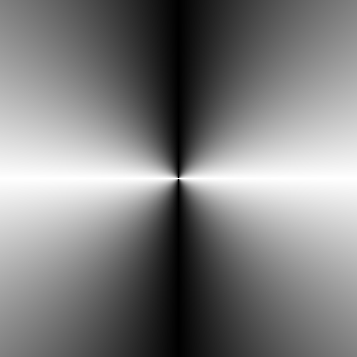
gray coloring

Map argument to hue

Just like the previous mapping, the color of a number is determined purely by its argument. This time we map the argument to the hue, while keeping the saturation and lightness maximum.

function ArgHue(z)
    hue = ((angle.(z)) ./ π .+ 1) .* 180
    return HSV.(hue, 1, 1)
end

## ArgHue (generic function with 1 method)

colors = ArgHue(plane(-1.0, -1.0, 1.0, 1.0));

This will produce the following coloring of the complex plane:

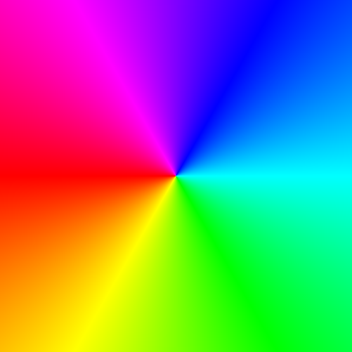
hue coloring

Map complex numbers to HSV colors

This is not just one mapping, instead it is a function that generate mappings. The hue is determined by the argument of the complex number, just like with the ArgHue mapping above, but this time the saturation and lightness are calculated from the modulus of the complex number. The calculation is influenced by two parameters, f1 and f2.

function CompHSV(f1, f2)
    function f(z)
        hue = ((angle.(z)) ./ π .+ 1) .* 180
        s = 2 .* atan.(( abs.(f1 .* z))) ./ π
        v = 1 .- 2 .* atan.(( abs.(f2 .* z))) ./ π
        return HSV.(hue, s, v)
    end

    return f
end

## CompHSV (generic function with 1 method)

colors = CompHSV(2.0, 0.5)(3 .* plane(-1.0, -1.0, 1.0, 1.0));

This will produce the following coloring of the complex plane:

hsv coloring

Generating the actual plot

The following function puts it all together. It receives the corners of the plotted region, the coefficient functions \(a\) and \(b\), the number indicating which convergent to calculate, and a coloring function. It will return the resulting image.

function plotCF(x0, y0, x1, y1, a::Function, b::Function, k::Int64,
                coloring::Function)
    z = plane(x0, y0, x1, y1)
    image = contfrac(a, b, k, z)
    return coloring(image)
end

## plotCF (generic function with 1 method)

Image no 17

function a(i::Int64, z)
    if i == 0
      return zero(z)
    end
    return z .* cis(π * i/2)
end

## a (generic function with 1 method)

function b(i::Int64, z)
    return zero(z) .+ i
end

## b (generic function with 1 method)

img = plotCF(-2.0, -2.0, 2.0, 2.0, a, b, 100, GrayReIm);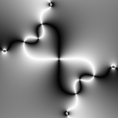

Image number 17

Image no 255

function a1(i::Int64, z)
    if i == 0
        return zero(z)
    end
    return cis.(π .* z)
end

## a1 (generic function with 1 method)

function b1(i::Int64, z)
  return (-1)^i .* z
end

## b1 (generic function with 1 method)

img = plotCF(-1.0, -.5, 1.0, 1.5, a1, b1, 100, ArgHue);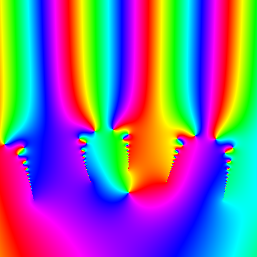

Image number 255

Image no 246

function a2(i::Int64, z)
    if i == 0
        return zero(z)
    end
    return i * cis.(-π * i/2) .* z
end

## a2 (generic function with 1 method)

function b2(i::Int64, z)
    return cis(-π*i/2) * i .+ z
end

## b2 (generic function with 1 method)

img = plotCF(-1.0, -.5, 1.0, 1.5, a2, b2, 100, CompHSV(2.0, 0.5));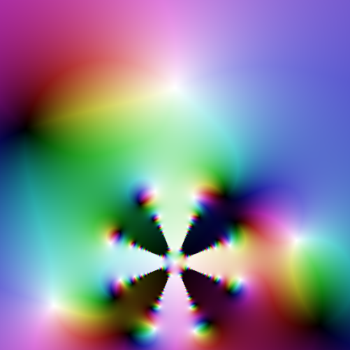

Image number 246