This has been bothering me for a while: is there a good simple way to apply a formula to rows of a data frame or table, where the formula would consume the rows as vectors?
Update: There is actually a very simple way to do it. See the next post.
Motivation
The section 3.3 of the Introductory Statistics with Randomization and Simulation contains the following example:
In the first case, we consider data from a random sample of 275 jurors in a small county. Jurors identified their racial group, as shown in the table below, and we would like to determine if these jurors are racially representative of the population. If the jury is representative of the population, then the proportions in the sample should roughly reflect the population of eligible jurors, i.e. registered voters.
| Race: | White | Black | Hispanic | Other | Total |
|---|---|---|---|---|---|
| Representation in juries: | 205 | 26 | 25 | 19 | 275 |
| Registered voters: | 0.72 | 0.07 | 0.12 | 0.09 | 1.00 |
While the proportions in the juries do not precisely represent the population proportions, it is unclear whether these data provide convincing evidence that the sample is not representative. If the jurors really were randomly sampled from the registered voters, we might expect small differences due to chance. However, unusually large differences may provide convincing evidence that the juries were not representative.
Although the book has the words “Randomization and Simulation” in the title, it does not talk about simulation for a goodness of fit test. Instead, it jumps straight into calculating \(\chi^2\) score, and then brings in the \(\chi^2\) distribution and goes on to find the p-value estimate from the table that is in the back of the book. This is, however, very easy to simulate. There is just one step that I wish was a bit simpler.
Simulation
We will make one basic assumption to make the simulation simpler: we will assume that the county, although small, is nevertheless large enough so that when we select a sample of size 275, the selections can be considered independent.
The question we are trying to answer here is: how would the samples look like if the jurors really were selected completely randomly from the population? We can easily get an answer to that by taking a bag with 100 pieces of paper, 72 of them labeled White, 7 labeled Black, 12 labeled Hispanic and 9 labeled Other. This bag will simulate the county population. Then we randomly sample 275 pieces of paper with replacement (since we assume that the individual selections can be considered independent).
A lot of very easy simulations of this type in R can be done with the mosaic
package. In class I usually start with two level factor variables (single
proportion), simulated either by sampling from a bag or using a loaded coin.
We will also use the tidyverse: first we will want forcats to make creating
an ordered factor easier, and later we will use more tidyverse packages to
analyze the results of the simulation.
library(tidyverse)
library(mosaic)
We need to prepare a “bag” from which we will sample. There are several ways to do this. For example, we can start by creating a list of labels to use. It is important to create the labels as an ordered factor, so later as we simulate the sampling, things will be always kept in the same predictable order.
In plain R, creating an ordered factor with a specific order requires a bit of
a boilerplate, but the forcats package makes this much easier. The only
thing that I find puzzling is that a function that is specifically designed for
creating factors with a specific order has an ordered parameter that defaults
to FALSE. Consistency … hobgoblin …. I mean, one of the great things
about the tidyverse is that unlike functions in base R, that are, as they say
in my country, “each dog different village”1, the tidyverse functions have a
consistent interface, but this seems to be going a bit too far.
labels <- fct_inorder(c("White", "Black", "Hispanic", "Other"), ordered=TRUE)We will also need a table of percentages that describe the population from which we sample. We can use the labels as names for the list entries, just to keep things a bit more organized.
percentages <- c(72, 7, 12, 9)
names(percentages) <- labels
percentages
## White Black Hispanic Other
## 72 7 12 9Now we are ready to create the bag that will represent the county population,
from which we will sample. We could also simply sample directly from the
labels variable, and use the percentages to specify the probability of each
of the labels, but let’s try to simulate the sampling from a bag with pieces of
paper as closely as possible.
bag <- rep(labels, percentages)
bag
## [1] White White White White White White White
## [8] White White White White White White White
## [15] White White White White White White White
## [22] White White White White White White White
## [29] White White White White White White White
## [36] White White White White White White White
## [43] White White White White White White White
## [50] White White White White White White White
## [57] White White White White White White White
## [64] White White White White White White White
## [71] White White Black Black Black Black Black
## [78] Black Black Hispanic Hispanic Hispanic Hispanic Hispanic
## [85] Hispanic Hispanic Hispanic Hispanic Hispanic Hispanic Hispanic
## [92] Other Other Other Other Other Other Other
## [99] Other Other
## Levels: White < Black < Hispanic < OtherNow we can sample from the bag. Sample 275 pieces of paper with replacement, and tally the results:
tally(sample(bag, 275, replace=TRUE))## X
## White Black Hispanic Other
## 204 19 30 22This is an example how the juror distribution could look like if the jurors were selected randomly.
Now we want to repeat this many times, and collect the results. The mosaic
package makes this really easy:
do(1000) * tally(sample(bag, 275, replace=TRUE)) -> selections
glimpse(selections)
## Observations: 1,000
## Variables: 4
## $ White <int> 191, 203, 192, 195, 212, 200, 209, 194, 195, 193, 207, …
## $ Black <int> 20, 24, 17, 17, 11, 17, 16, 18, 19, 21, 13, 15, 25, 19,…
## $ Hispanic <int> 37, 25, 36, 33, 35, 28, 32, 32, 36, 37, 35, 25, 32, 28,…
## $ Other <int> 27, 23, 30, 30, 17, 30, 18, 31, 25, 24, 20, 34, 20, 35,…As we can see, each row of the selection data set is a summary of a simple
random sample of size 275 from the simulated population. We can perhaps see it
better when looking at the first few rows:
head(selections)## White Black Hispanic Other
## 1 191 20 37 27
## 2 203 24 25 23
## 3 192 17 36 30
## 4 195 17 33 30
## 5 212 11 35 17
## 6 200 17 28 30\(\chi^2\) scores
Now that we have a large number of samples that are randomly selected from the given population, we need some way to compare the observed sample with all these simulated samples. We want to find some way to rank each sample, that will tell us how far each sample is from an ideal sample that has exactly the same proportions of each category as the population itself.
This is usually done with so called \(\chi^2\) scores. For each category, we want to compare the frequency of that category in the sample with the expected frequency of the category. Since each category has different expected frequency, the distributions of the frequencies will be different. To be able to safely combine and compare the frequencies in different categories, we need to divide the difference between the sample frequency and the expected frequency by the standard deviation, which, in this case, can be calculated as the square root of the expected frequency. That means we actually calculate the z-score of each sample frequency.
To combine the z-scores for all categories together, we need to make them non-negative, and then add them together. For the \(\chi^2\)-score, we make them non-negative by squaring them, so the score is then calculated as \[\chi^2 = \sum \frac{\left(\text{sample frequency} - \text{expected frequency}\right)^2}{\text{expected frequency}}\] Let’s start by calculating the \(\chi^2\) score of the observed sample. To start with we need to find the expected frequencies. The sample size is 275, and the population percentages for each category we already entered:
percentages## White Black Hispanic Other
## 72 7 12 9The expected frequencies will then be
expected <- 275*percentages/100
expected
## White Black Hispanic Other
## 198.00 19.25 33.00 24.75We also need to enter the frequencies of the observed sample:
observed <- c(205, 26, 25, 19)
names(observed) <- labels
observed
## White Black Hispanic Other
## 205 26 25 19Then the \(\chi^2\) score of the observed sample is simply
observed_chi_square <- sum((observed - expected)^2/expected)
observed_chi_square
## [1] 5.88961Now we need to do the same calculation for each of the simulated samples. This is where things get complicated.
Ideally, we would just map the formula over the data set, row wise. However, I
was not able to find a way to do this. A logical place to look at would be the
purrr package. It does provide some ways of
mapping a formula over rows, however, as far as I can tell, none of them will
let me use rows as vectors. From the description it would seem like pmap
should do it, but I was unable to make it work, and none of the examples that I
found on the web seem to apply to this situation. It seems that there is no
way to use the whole row as a vector in pmap. As far as I can tell, you
need to specifically enter each of the arguments in pmap, using numbered
codes like ..1, ..2, and so on.
I can do for example this:
selections %>%
    mutate(chisq = pmap_dbl(., ~sum((c(..1, ..2, ..3, ..4) -
                                 expected)^2/expected))) %>%
    head()
## White Black Hispanic Other chisq
## 1 191 20 37 27 0.9660895
## 2 203 24 25 23 3.3614719
## 3 192 17 36 30 1.8311688
## 4 195 17 33 30 1.4220779
## 5 212 11 35 17 7.0735931
## 6 200 17 28 30 2.1544012which is fairly close to what I am looking for, but the c(..1, ..2, ..3, ..4)
will quickly get unwieldy and error prone with larger number of categories.
Ideally, I would like to be able to do something like
pmap_dbl(selections, ~sum((.row - expected)^2/expected))but there does not seem to be any way to do this.
One way is to transpose the data frame - it is way easier to map things over columns than over rows. This will work nicely:
selections %>%
    mutate(chisq = transpose(.) %>%
           simplify_all() %>%
           map_dbl(~sum((.x - expected)^2/expected))) %>%
    head()
## White Black Hispanic Other chisq
## 1 191 20 37 27 0.9660895
## 2 203 24 25 23 3.3614719
## 3 192 17 36 30 1.8311688
## 4 195 17 33 30 1.4220779
## 5 212 11 35 17 7.0735931
## 6 200 17 28 30 2.1544012or, equivalently,
selections %>%
    mutate(chisq = transpose(.) %>%
           map_dbl(~sum((as_vector(.x) - expected)^2/expected))) %>%
    head()
## White Black Hispanic Other chisq
## 1 191 20 37 27 0.9660895
## 2 203 24 25 23 3.3614719
## 3 192 17 36 30 1.8311688
## 4 195 17 33 30 1.4220779
## 5 212 11 35 17 7.0735931
## 6 200 17 28 30 2.1544012The problems I have with this approach are:
- It requires a “nested” pipe (or a mess of nested parentheses which is something that students learning R for the first time have trouble with).
- It introduces two additional concepts (transposition and either
simplify_alloras_vector) that have nothing to do with the already pretty complicated topic of goodness of fit test.
Finishing the test
Let’s quickly finish the comparison of the observed sample frequencies with the simulated sample frequencies. First, let’s actually use one of the less than ideal ways to calculate the \(\chi^2\) scores:
selections %>%
    mutate(chisq = transpose(.) %>%
           map_dbl(~sum((as_vector(.x) - expected)^2/expected))) ->
    selections_with_chisq
Then we plot the \(\chi^2\) scores of all the simulated samples, and mark the observed \(\chi^2\) on the plot with a vertical line.
gf_histogram(~chisq, data = selections_with_chisq) %>%
    gf_vline(xintercept = observed_chi_square, color="red")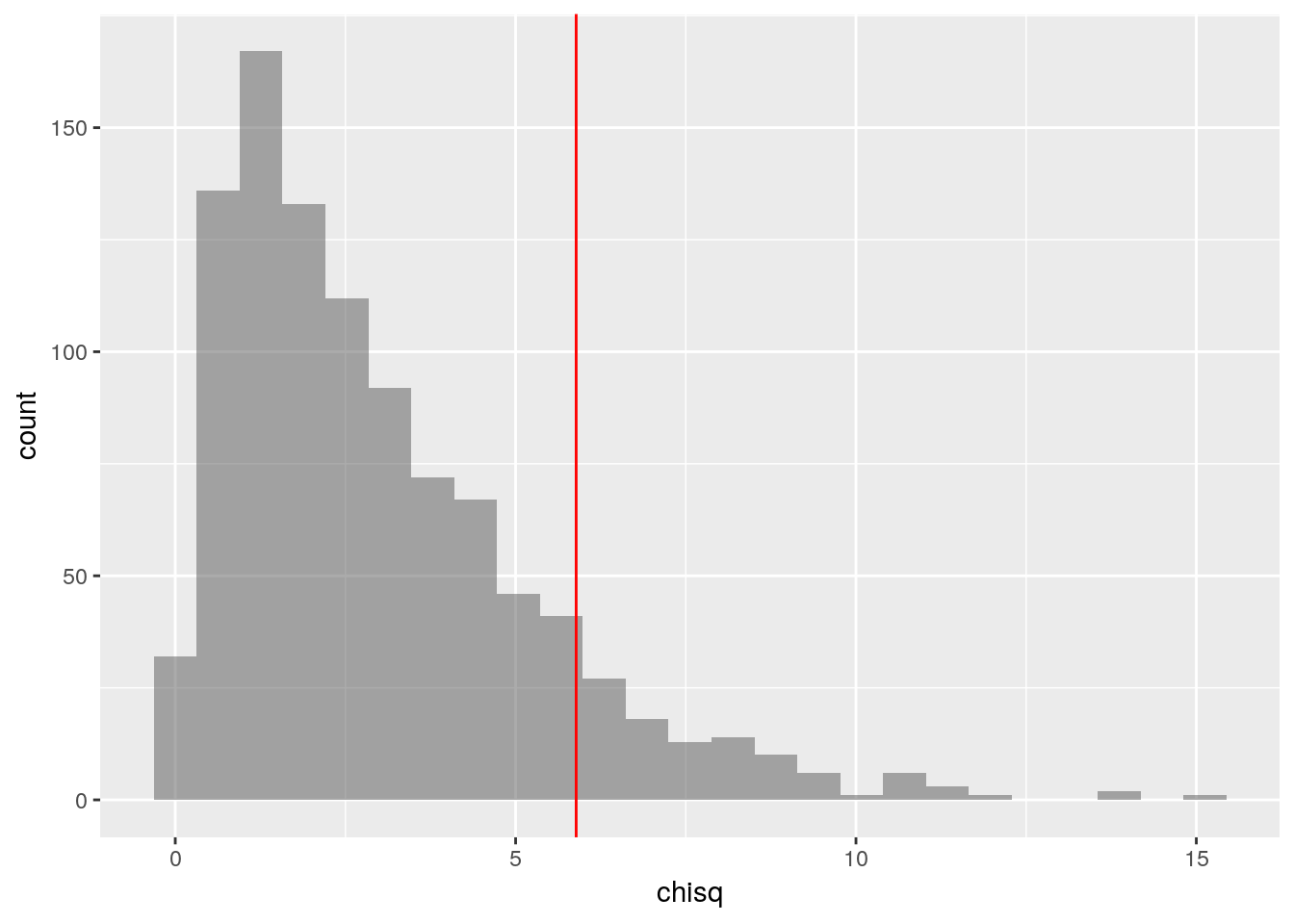
We can then easily answer the question “how many of the 1000 simulated samples had a \(\chi^2\) score greater than or equal to the observed \(\chi^2\) score?”
count(~(chisq >= observed_chi_square), data = selections_with_chisq)## n_TRUE
## 110I don’t understand it either, but at least it rhymes in Czech.↩